Taking The Sting Out Of Cryptocurrencies

Introduction

In the face of structurally slower long-term economic growth caused by aging populations, shrinking work forces, and weak capital formation and productivity – as well as the impact of the Pandemic – central bank balance sheets and government borrowings have exploded. The result has been to undermine national currencies through inflation and the potential for competitive currency depreciation. In this scenario, alternative, decentralised currencies, free of policy manipulation – such as cryptocurrencies – have become increasingly attractive.

However, cryptocurrencies are still a developing asset class and are extremely volatile. This note will show how – using an appropriate trading strategy – one can significantly reduce the volatility of cryptocurrencies while simultaneously enhancing their returns.

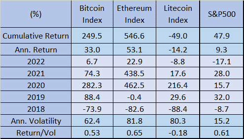
Performance of Cryptocurrencies

The historical returns from cryptocurrencies have been staggering. Since the beginning of 2018 to 20 May 2022, Bitcoin and Ethereum, for example, have risen by nearly 250% and 550%, respectively, compared to 48% for the S&P 500 (see chart and table below). However, although returns have been stellar, cryptocurrencies have also experienced enormous volatility – in 2018, Bitcoin fell by more than 70%.

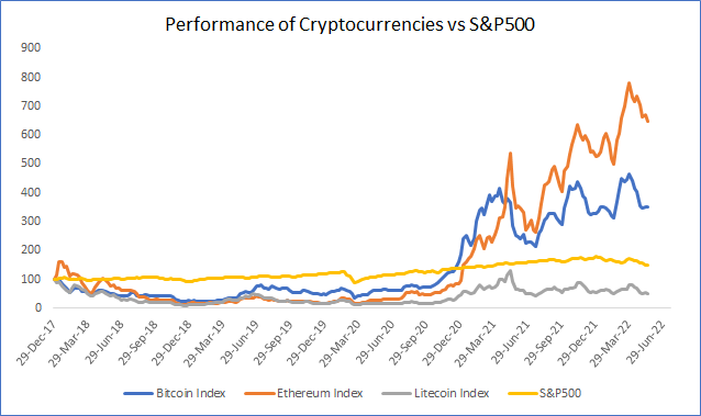
Modeling Cryptocurrencies

Unlike equities, cryptocurrencies are more difficult to value because they do not produce earnings or dividends. However, one might still be able to value cryptocurrencies in relation to macroeconomic and market factors if one can establish that there is a meaningful long run relationship. If so, then one can calibrate these relationships in order to find a model that best fits the historical variation in cryptocurrency prices, which can then be used to minimise volatility and maximise returns.

A number of factors spring to mind that may be able to explain the variation in cryptocurrency prices. Gold is one, as it is also seen as an alternative currency. Bonds are another, as a rising yield becomes more attractive relative to another asset that doesn’t generate any income. Equities could also be an important factor as a rising equity market reflects increasing risk appetite, which is likely to spill-over into the cryptocurrency market. The dollar is probably one of the most important factors, since the raison d’etre of cryptocurrencies is the fear of currency debasement. Lastly, the VIX volatility index might be significant, as cryptocurrencies could be a hedge against uncertainty.

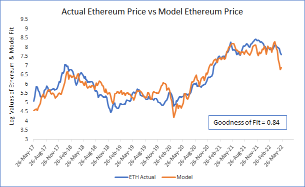
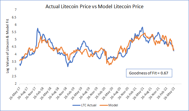
These factors can be used in a multiple regression which estimates a line of best fit between the cryptocurrency price and the factors. The slope of this line on each factor is the factor beta, which gives a measure of the influence of the factor on the cryptocurrency. We can combine these betas to estimate a model price of the cryptocurrency. The charts below compare the actual (log) price of Bitcoin, Ethereum and Litecoin, with their respective model prices. We can see that in the last five years, the model price fits the actual data very closely, with a “goodness of fit” of 0.89 (the maximum being 1.0) for Bitcoin, 0.84 for Ethereum and 0.67 for Litecoin.

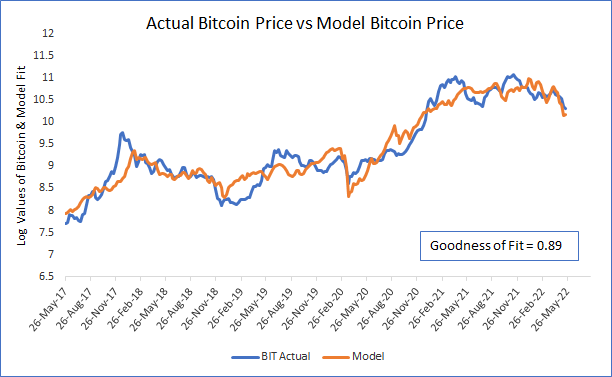
Factor Contributions

Of the factors used in the model, which ones are the most important? We can see in the chart below that the largest beta is on the Dollar, followed by the S&P500 and Bond yields.

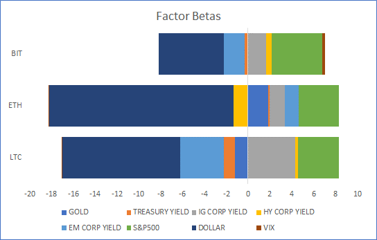
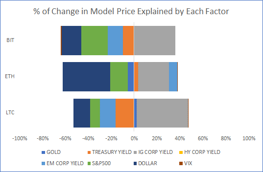
However, it doesn’t matter how big the beta is, if the factor doesn’t move very much then it’s not going to have much influence in the model. So one has to look at how much the factor has moved as well, and the combination of the two will give a handle on the contribution of each factor over a particular period of time. The next two charts show this, and one can see that in the twelve weeks to 20 May 2022, the most important factors contributing towards the change in the Bitcoin model price, for example, were the investment grade corporate bond yield, the S&P500 and the Dollar.

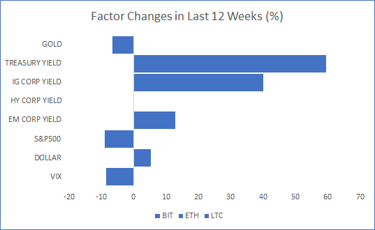
Cryptocurrency Trading Strategy

Since there is a close long run relationship between the actual and the model cryptocurrency price, then, in theory, any divergence between the two should only be temporary, and the spread between them should be mean-reverting. This is indeed the case as can be seen in the charts below.

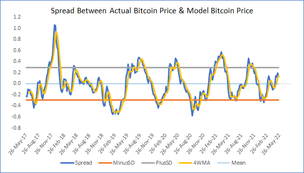
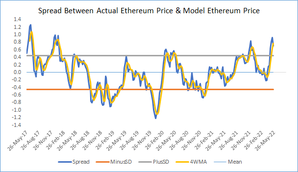
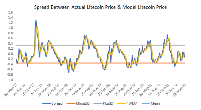
Since the spreads are mean-reverting, if the actual price is above the model price then the cryptocurrency is over-valued and if the actual price is below the model price then the cryptocurrency is under-valued. A strategy then presents itself: if the actual price is excessively above the model price, sell the cryptocurrency; and if the actual price is excessively below the model price, buy the cryptocurrency. The trades are unwound when the spread mean-reverts.

Cryptocurrency Strategy Performance

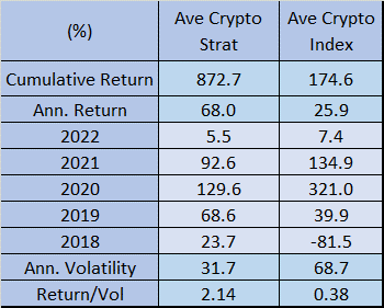
The results of this strategy are very promising, as shown in the chart and table below. An equally weighted portfolio of the three cryptocurrency indices, over the period 1 Jan 2018 to 20 May 2022, would have produced an annualised return of 25.9% with a 68.7% annualised standard deviation (volatility). On the other hand, an equally weighted portfolio of the three cryptocurrency strategies, over the same period, would have produced an annualised return of 68% with an annualised volatility of 31.7%. So the cryptocurrency strategy would have reduced cryptocurrency volatility by more than half and more than doubled cryptocurrency returns in the process.

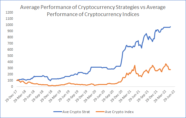
Conclusion

In a world of policy-induced monetary debasement, de-centralised digital assets such as cryptocurrencies, are increasingly attractive. But they come with significant volatility. One way to minimise this volatility while enhancing returns is to find macroeconomic and market factors that influence cryptocurrency prices, and trade the relationship between them. The results are very appealing.

Thank you for reading my note; I hope you found it interesting.

Data source: Federal Reserve. Results are estimates.