


mikkelwilliam
Co-Authored with Total Return Investor
Revisiting Julia 2023
The concept of an All-Weather Portfolio – a portfolio that can perform satisfactorily in any market conditions, without any need for buying or selling – is not a new one. The “60/40” portfolio – 60% stocks, 40% bonds – is an idea that’s been around since at least the middle of the last century. According to the 60/40 theory, the prices of stocks and bonds tend to vary inversely, with one going up when the other is going down, so a portfolio balanced between the two should maintain a more even keel over time than pure stock or bond portfolios. Very broadly, the historical data bears out the 60/40 view. (For statistical details, please see our original article, The Search for an All-Weather Portfolio.)
Of course, if keeping an even keel is the objective, the obvious and immediate question is, does the 60/40 portfolio do the best possible job of it? Putting 60% of one’s capital in a broad stock market fund, 40% in a broad bond market fund, and expecting optimal performance, seems almost too easy (although Vanguard’s highly respected Vanguard Balanced Index Fund Inst (VBIAX), which implements the 60/40 strategy by simply following two broad-market indices, continues to be a respectable competitor). And indeed, as can be seen on the websites PortfolioCharts.com, LazyPortfolioETF.com, and OptimizedPortfolio.com, dozens of proposals have been made for better AWPs than the 60/40. In our preceding article, we set up a uniform framework for evaluating these AWPs, evaluated some of the most famous of them, and offered a statistically superior alternative of our own, “Julia.”
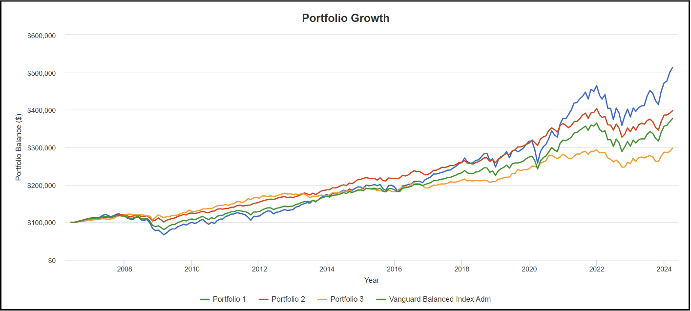
Here’s a chart which gives the flavor of the results from our previous article. It employs Portfolio Visualizer.com, an outstanding website (free for the basic version) which provides tools for portfolio evaluation as well as a number of other financial metrics.
Portfolio Visualizer
It’s worth taking a few minutes to understand the results here. Portfolio 1, the blue line, is what we call “Buffett’s Widow”, based on Warren Buffett’s onetime remark that if he were recommending a portfolio for his wife in the event of his death, it would be 90% a broad market index fund (we’ve used Vanguard Total Stock Market Index Fund ETF Shares (VTI)) and 10% a short-term treasury bill fund (we’ve used SHY, the iShares 1-3 year Treasury bond index.) Portfolio 2, the red line, is Julia as we presented it in our original article, which we’ll discuss a little further below. The green line is the classic 60/40 portfolio as represented by Vanguard’s VBIAX fund; and Portfolio 3 is the “Permanent Portfolio” propounded by Harry Browne (Libertarian candidate for President, 1996 and 2000.) Our original article analyzed several other AWPs, such as the Ray Dalio portfolio as popularized by Tony Robbins, but Portfolio Visualizer only allows comparison of three portfolios at a time plus an index, so you’ll have to consult our prior article for further information.
It’s helpful to consider the statistical analysis of this graph as presented by Portfolio Visualizer, for our test period of June 2006 to the present. (We start in June 2006 because that is the inception date of one of Julia’s core components – VIG, the Vanguard Dividend Appreciation index, and includes the important stress test of the Global Financial Crisis of 2007-9):
|
Portfolio |
Initiated 6/2006 |
CAGR |
Balance 3/2024 |
30 Year Projection |
Maximum Drawdn |
Sharpe Ratio |
|
1-Buffett’s Widow |
100,000 |
9.60% |
512,878 |
1,564,288 |
-45.95% |
0.62 |
|
2-Julia |
100,000 |
8.37% |
397,458 |
1,114,993 |
-18.95% |
0.87 |
|
3-Browne |
100,000 |
6.39% |
297,813 |
641,245 |
-15.85% |
0.70 |
|
Vanguard 60/40 |
100,000 |
7.72% |
376,738 |
930,873 |
-32.45% |
0.66 |
Portfolio Visualizer and Authors’ Projection
Consider what these statistics show. Yes, Portfolio 1 (“Buffett’s Widow”) has the superior Compound Average Growth Rate (CAGR), appearing as the top line on the graph, but at the price of a horrendous 45.95% drawdown during the test period (note the pandemic year 2020.) Also note how long Portfolio 1 lagged the others, especially Julia, in the aftermath of the Global Financial Crisis. (This would probably be of little concern to Mrs. Buffett, but consider the effect on a retiree of modest means setting out to follow the 4% withdrawal rule.) Yes, Portfolio 3 (Browne’s “Permanent Portfolio”) has a maximum drawdown of only 17.20%, but at the expense of a CAGR of only 6.39%, with a final balance of only $297,813 over the test period, the worst of all the AWPs in the group. (The effect of compounding becomes particularly stark when projected out to 30 years.) The 60/40 portfolio comes out somewhere in the middle. But the Sharpe ratio – the ratio of growth to downside risk – comes out massively in Julia’s favor. This one summary table can’t tell the whole tale, but as of last year’s publication, we believe it was indicative of a substantial advantage in favor of the way Julia is constructed.
And how was Julia constructed? As we explained in our preceding article, the crucial difference from the traditional 60/40 was to break the stock component down into three parts:
|
Steady Income and Earnings Growth |
(VIG) Vanguard Dividend Appreciation Index |
16% |
|
Dynamic Growth and Innovation |
(QQQ) Invesco Nasdaq 100 |
16% |
|
Stable, Defensive Slow Growth |
(XLP) Consumer Staples Sector SPDR (XLV) Health Care Sector SPDR (XLU) Utilities Sector SPDR |
6% 6% 6% |
|
50% |
||
The net result of this division was to improve the performance of Julia’s stock component by almost 1% over pure VTI. As shown in the table above, even a tiny percentage difference in CAGR can produce dramatic differences in net result, when compounded over a period of two or three decades.
The rest of Julia, as we presented it last year, was designed less systematically, because it was TRI’s actual working portfolio at the time, and displays all the quirks that distinguish real portfolios from idealized virtual creations. Here is TRI’s personal account of how Julia became his personal portfolio:
After a hectic 2020 COVID year of buying and selling (both individual companies and funds), at age 74 I realized that I was not getting any younger or smarter, and that my wife had neither the knowledge nor inclination to manage such a portfolio. So, in late 2020 I reversed course. Consolidating the winners and abandoning the losers, I ended 2020 with an 11.3% gain, allocated as follows: 25% in a single total US market stock fund, 40% in a single aggregate bond fund, 20% in a short term Treasury fund, and 15% in bank CDs and brokerage cash. It was not a bad place to catch my breath, but was clearly too conservative to be a permanent solution. By the spring of 2021, the hunt was on for something better.
I became fascinated with Ray Dalio’s well-publicized AWP (see our original article for its details), and gradually began assembling it. Initially things went well, but as 2021 wore on, I suspected that there were significantly better AWP possibilities. That fall, oriented more to Portfolio Adviser evaluations, I exited Dalio’s recommended DBC broad commodities at a very nice profit, exited GLD at a wash, and cut back significantly on my march towards Dalio’s recommendation for 40% in long term Treasuries (thank goodness!)
At the beginning of 2022, I was holding roughly equal 22% portions of long term Treasuries and aggregate bonds, a 6% dollop of inflation protected Treasuries in a nod to inflation (which was obviously heating up), and 42% in stocks, mostly in a broad market stock fund. The remaining 8% was equally divided between short term Treasuries and cash. Over the course of 2022, the broad stock fund was gradually allocated to more focused alternatives, as we detailed in last year’s article. By early 2023, Julia as described in last year’s article was essentially in place.
While Julia 2023 was a significant improvement upon the “usual suspects” in the AWP lineup, we believe that it can still be improved. We begin with an important distinction that often lurks in the background of portfolio analysis, but is seldom if ever clearly drawn.
The Distinction Between Working and Reserve Assets
We now draw a fundamental distinction between a person’s Working and Reserve assets. (Financial assets; real property is beyond the scope of this discussion.) Working assets, as we now think of them, are invested with the purpose of earning a significant favorable return, relative to inflation. Reserve assets are focused on the preservation and utilization of wealth. For instance, a checking account balance (and some people prefer to keep a large one) is a Reserve asset. It’s generally not intended to generate a serious return; it’s intended to pay upcoming bills and ongoing expenses. Many financial advisors suggest enough ready cash to sustain a family for six months to a year in case of unexpected emergencies; again, the point is to have a completely liquid reserve, not to maximize return on investment. Simple “walking-around money” is also a reserve. Conceptually, reserve assets should be completely segregated, mentally if not physically, from working assets that are intended to produce a positive return.
But exactly where is the dividing line between Working and Reserve assets? Well, money in one’s wallet or under the mattress (at least in a completely secure and inflation-free world) would probably be the clearest example of a reserve asset: “pure cash,” legal tender. SHY, the one-to-three year Treasury bill ETF (currently yielding around 3.2% in an environment where the last reported CPI was… 3.2%), can on rare occasions offer a positive return (though not in the long run.) BIL, the one-to-three month Treasury bill ETF, currently yields a little more than 5%, but that yield will come down quickly assuming the Fed begins to cut the fed funds rate. Where to draw the line?
Well, there is no bright line to draw. Bond funds come in all durations. While it is classified as a bond fund, SHY is a well-known, highly-liquid, short-duration instrument widely regarded as a good “parking place” for cash – because it behaves much more like cash than longer duration bonds that offer the potential for at least some real return. Without further ado, or any pretense of deep knowledge of the bond market, we arbitrarily set the inflation-adjusted real return of SHY as the boundary line between Reserve and Working assets. We’ll call SHY or any of its many relatives capital-C Cash.
The important point to appreciate is how the amount of reserve assets held affects the rate of return on total assets. Consider the following table of total asset returns during our test period, beginning with the 14% in reserve assets that TRI reports above, and then reducing the reserve assets to 7% and 0%:
|
Total Assets 6/2006 |
% Reserve Assets |
% Working Assets |
CAGR of Total Assets |
Balance 3/2024 |
30-Year Projection |
Maximum Drawn |
Sharpe Ratio |
|
100,000 |
14 |
86 |
7.59% |
366,397 |
897,754 |
-19.87% |
0.86 |
|
100,000 |
7 |
93 |
8.11% |
399.134 |
1,037,471 |
-21.19% |
0.86 |
|
100,000 |
0 |
100 |
8.61% |
433,201 |
1,191,501 |
-22.48% |
0.86 |
What we see here is the classic financial concept of risk/reward trade-off at work. Reserve assets are held in very low-risk, low-reward instruments (Cash); working assets such as TRI’s Julia portfolio produce higher reward in return for being more vulnerable to market fluctuations. The less risk one chooses to take (by holding a greater percentage of reserve assets), the fewer dollars a working portfolio has with which to earn its projected return. Since Cash produces a lower return than any of the other assets normally held in a working portfolio, holding more Cash will inevitably result in a lower return on total assets that a working portfolio can produce. However, the Sharpe ratio, reward gained for each unit of risk taken, stays exactly the same.
What’s the correct percentage of reserve assets to hold? The answer will vary for each individual. Some people are simply more risk-averse than others (as with the authors of this article.) Some people may reasonably anticipate a greater possibility of emergency expenses in the future. Some may choose to decrease the percentage of assets held in reserve as total assets increase, while others may not. There is simply no accounting for financial taste.
But one important advantage of segregating reserves from working assets is that it allows a rather precise determination of the costs of safety. TRI describes his personal situation:
I did not own Julia until early 2023. However, if I had held Julia since June, 2006, then our back test could be used to analyze the costs of the 14% I now hold in reserves against the costs or benefits of other possible percentages.
For example, if I had held only half of that 14% in reserves over the last 18 years, then my wife and I would be able to safely move into the luxury retirement village of our dreams three years sooner. As it is, actuarial tables and Monte Carlo simulations show that, should we move there in 2024, we would not be completely out of the woods for going bankrupt in our late-90s, in the unlikely but possible scenario where we live that long. Since going bankrupt with one’s personal belongings set out at the curb at that age is the worst imaginable end to lives that have gone reasonably well so far, we choose not to run that risk. So we will check back in a few years, when we are closer to the finish line. An additional three years of cooking, cleaning, home maintenance, yard work, etc. was the cost to us of holding 14% rather than 7% in reserves since 2006. That is as precise and vivid an example of the cost of one level of reserves vs another as can be drawn.
Such hindsight is perfect, but what about going forward? I am not comfortable going forward with only 7% in reserves, because I am not confident the next 18 years will go as well for us personally as the last 18 have. In fact, I will be quite surprised if they do. Age 96 is not yet, and probably never will be, the new 78. I am quite ignorant about the costs of various hazards we might confront—e.g., the possible costs of prescription drugs over and above what a Medicare drug plan will cover, the average size of health emergencies occurring overseas and hence beyond Medicare coverage, or the average amount not covered by homeowners insurance for natural disasters in our area. There could be black swan possibilities that are not even remotely on our radar. Fortunately, there are online sites with disinterested experts whose job is to know and quantify such things. Relying heavily upon their estimates, I tentatively settle upon a range of 12-22% going forward for persons in our circumstances.
Whatever the size of the reserves an individual settles upon, however, the authors believe that it’s important not to muddy the distinction between reserve and working assets by putting reserve assets into a working portfolio. Consider Browne’s Permanent Portfolio, probably the most famous example, which specifies 25% held in Cash. Compare the results if we take Cash entirely out of the Permanent Portfolio, or reduce it to a more modest 10%, while maintaining equal proportion between the other elements.
|
Permanent Portfolio, 6/2006-3/2024 |
Initial Balance |
Final Balance |
30-Year Projection |
CAGR |
Maximum Drawn |
Sharpe Ratio |
|
Browne’s Original: 25% each VTI, TLT, GLD and Cash |
100,000 |
300,254 |
641,245 |
6.39% |
-17.20% |
0.69 |
|
No Cash in the PP: 33.3% each VTI, TLT and GLD |
100,000 |
385,594 |
978,686 |
7.90% |
-21.45% |
0.69 |
|
30% each VTI, TLT, GLD, with 10% Cash |
100,000 |
348,103 |
823,309 |
7.28% |
-19.73% |
0.69 |
That’s pretty dramatic! Now, perhaps Browne was really so risk-averse that he was willing to give up very large amounts of money to maintain 25% in reserve funds. Perhaps he had simply not considered how differences in individual circumstances can produce great variations in the amount needed in reserves. We suspect, however, that he was simply entranced by the symmetry of a portfolio divided into equal fourths. Had he started out from a distinction between working and reserve assets, contemplating the reduction of return introduced by each incremental increase of reserves, he might well have ended up allocating less to Cash. (The 30-30-30-10 allocation brings Browne up to almost exactly the CAGR of the classic 60/40 portfolio, with a far superior maximum drawdown.) In any case, we believe that mentally separating the working portfolio from the desired amount of reserve assets will have a clarifying effect on the thinking of most investors.
While we’re on this subject, we should note that the “Buffett’s Widow” AWP – 90% VTI, 10% SHY – also suffers from the same problem of mixing Working and Reserve assets. Is 90-10 really the ideal match for every investor’s risk tolerance? Mrs. Buffett might still want to set aside 10% ready Cash from her working portfolio, but individuals with a more modest amount of assets or a more conservative temperament might want considerably more. Again we see that the composition of the working assets, and the percentage of reserve assets, are two different questions. Buffett’s advice might more helpfully be generalized as “Put all your Working assets in a broad market fund like VTI, after setting aside the amount of Reserves that will make you feel comfortable.”
The Further Evolution of Julia
TRI: A year ago, Julia and my personal portfolio were essentially identical. Since then, as mentioned above, I have conceptually (but not physically) moved SHY and SNOXX ETFs into a separate reserve portfolio. I have also permanently closed the TIP ETF, with most of the proceeds going to provide a boost to reserves. Not only did I want to boost the reserves; I also could not see how TIP was serving any portfolio purpose distinct from AGG. Bottom line: TIP is gone, and our reserves now contain 14% of our total financial assets.
Excluding the reserve assets SCHO, SNOXX, and TIP brings Julia to an allocation of 56% stocks, 44% bonds. This led the authors to wonder what would happen if we took Julia the rest of the way to 60/40, while retaining the division of the stock portion described above, and simplifying the bond portion to contain only the aggregate and long-duration bond funds. Further trial-and-error experimentation in Portfolio Visualizer also led us to eliminate XLU, the weak sister among the three SPDR defensive sector funds. The final result was a greatly simplified Julia consisting of QQQ, 20%; VIG, 20%; XLP, 10%, XLV; 10%; TLT, 20%, and AGG, 20%.
Let’s start with a straight-up comparison of the new 60/40 Julia to the classic 60/40 (as embodied in Vanguard’s VBIAX fund.) Results are updated through March 31, 2024.
|
Portfolio |
Initiated 6/2006 |
CAGR |
Balance 3/2024 |
30-Year Projection |
Maximum Drawn |
Sharpe Ratio |
|
Julia 60/40 |
100,000 |
9.32% |
490,000 |
1,448,724 |
-21.89% |
0.89 |
|
Vanguard 60/40 |
100,000 |
7.72% |
376,738 |
930,873 |
-32.45% |
0.66 |
We confidently draw some conclusions from this result. The classic 60/40 portfolio is a venerable contender among AWPs, and outperforms a number of recent, more exotic designs. But using a broad or total market index like SPY or VTI for the entire stock component of a 60/40 portfolio fails to separate the wheat from the chaff. By using a balanced selection of established dividend payers, dynamic growth companies, and reliable defensive sectors (VIG, QQQ, and XLP/XLV), Julia tends to capture the more dependable earnings growers of the broad market, which are on balance the better performers. It tends to exclude the dinosaurs, the large-cap companies that are adrift or in decline.
As a result, Julia has a better compound average growth rate, holds up better in “bad weather”, and produces greater returns for the risk taken. The division of Julia’s bond component between a broad market fund (AGG) and long-term Treasuries (TLT) may have a similar benefit, but we take no position on the question – it is a subject for further research. Overall, however, we think a 60/40 portfolio with a segmented stock component clearly outperforms an undifferentiated broad market index.
And how does Julia of 2024 perform against the 2023 model? To answer this question, we must remember that Julia 2023, as described by TRI, contained a built-in 14% allocation to reserve assets. The only way to make an apples-to-apples comparison of Julia 2024 and Julia 2023 is to look at the total return for an investor who sets aside 14% of his/her total wealth in reserve assets, and then compare the results. While we’re at it, we can also check the results for an investor who holds 86% in VBIAX, the Vanguard 60/40 fund, and the same 14% in reserve assets. Portfolio Visualizer gives us the following results for our test period:
|
Total Assets |
Initiated 6/2006 |
CAGR |
Balance 3/2024 |
30-Year Projection |
Maximum Drawn |
Sharpe Ratio |
|
1-86% Julia 2024, 14% reserve assets |
100,000 |
8.77% |
447,663 |
1,245,300 |
-21.02% |
0.90 |
|
2-Julia 2023, 14% reserve assets built-in |
100,000 |
8.37% |
419,052 |
1,114,993 |
-20.04% |
0.88 |
|
3-86% Vanguard 60/40, 14% reserve assets |
100,000 |
7.72% |
332,834 |
930,873 |
-27.33% |
0.67 |
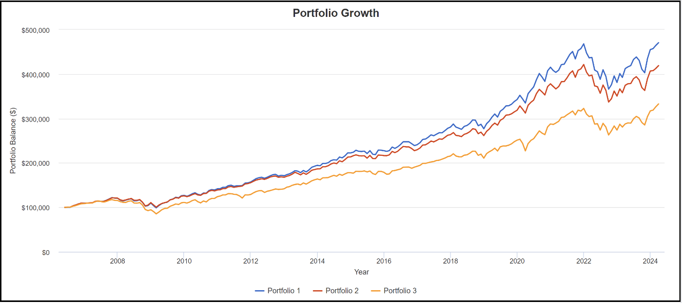
Portfolio Visualizer
And so, on equal footing, Julia 2024 represents an incremental improvement from Julia 2023, with slightly better return for risk taken and slightly higher long-term return, at the expense of slightly higher potential drawdown. Either version leaves classic 60/40 with undifferentiated stock and bond components in the dust. But the structure of Julia 2024 is certainly simpler and more intuitive than Julia 2023.
And besides the slight optimization, we believe that the separation of Working and Reserve assets makes Julia 2024 much easier to conceptualize and manage. Suppose an investor wants to keep maximum drawdown to less than 20%, the generally-accepted definition of a bear market. Fine; a little trial-and-error with Portfolio Visualizer will reveal that keeping 20% in reserve assets reduces maximum drawdown to 19.87%. Suppose the investor wants a CAGR of 9% (which according to the rule of 72, will double working assets every 8 years); Portfolio Visualizer says that 10% in reserve assets will allow that result to be achieved (at the price of a 21.79% maximum drawdown.) In return for a little work, the structure of Julia 2024, along with completely segregated Working and Reserve assets, allows (or challenges) the investor to decide exactly what risk/return trade-off they prefer.
TRI again: Making substantial alterations to a virtual portfolio is a snap, but making them to a real one is harder. I am en route towards full implementation of the new Julia, but am not there yet. As of April 1, my investment portfolio is QQQ, 18.9%; VIG, 19.2%; XLP, 10%, XLV, 10%; TLT, 20%; and AGG, 21.9%. The remaining swap of excess AGG funds for more QQQ and VIG is on hold until the two stock ETFs take a significant dip. As for an appropriate level of reserves, our current 14% is towards the low end of the 12-22% mentioned above, but I feel comfortable with it. I have no plans to move it either lower or higher.
I have made a few minor, judgment-based rebalancing trades over the last twelve months, the details of which are not worth recounting. More importantly, I have decided that at most I will make only such minor, selective rebalancing moves. This policy will continue as long as I manage the family portfolio. If at some future date my wife has to take over, then restructuring and rebalancing will immediately and permanently end. Like many SA spouses, she has no knowledge of nor interest in the markets. This has been a major factor in my search for a portfolio that at some future date could well become completely hands-off.
This raises the whole subject of periodic portfolio rebalancing. Portfolio Visualizer defaults to rebalancing Julia annually—no muss, no fuss. In contrast, rebalancing an actual portfolio is more tedious, and can carry harmful tax consequences. Frankly, it is not clear that even a complete failure to rebalance would be all that bad; it could even be an improvement. A Portfolio Visualizer test shows that when the Rebalancing option in Julia is set to None, its max drawdown increases less than 3%, while its CAGR increases 0.7%, over the entire 18-year test period! The Sharpe ratio is unchanged. On an initial investment of $100k, the un-rebalanced portfolio’s value increases $60k more than the value of one that is rebalanced annually. Extrapolate those results to the next 18 years, and the level of risk creep is simply not worth fretting over. The received wisdom regarding the necessity of rebalancing needs much closer examination. Could it be that the market itself does a better job of rebalancing than a numeric formula that dictates always holding to a percentage allocation that is exactly the same?
Conclusions
- The classic 60/40 portfolio sets a risk/return baseline that any AWP should be able to match, although as we demonstrated in our previous article, many well-known proposals for AWPs fail to beat the return of 60/40, involve greater risk, or make claims based on cherrypicked time periods.
- A 60/40 portfolio such as Julia that uses a segmented selection of ETFs within its stock component produces results that are clearly superior to using a broad market index.
- Investors should draw a sharp distinction between Working assets, i.e. assets intended to produce a return measurably above inflation, and Reserve assets, i.e. assets set aside for emergencies and everyday transactions, that are not primarily intended to produce investment-like returns.
- AWPs should contain only Working assets, and be evaluated only on their investment performance; Reserve assets (“Cash”) should not be included in AWPs. Once investors decide what percentage of their total assets should be set aside as Reserves, they can evaluate the AWP they prefer based purely on performance measures, and allocate the remainder of their assets to it accordingly.
- Julia 2024 provides the best risk/reward proposition of any AWP in the broad tradition of 60/40 allocation.
Postscript
It occurs to us that Julia may not be the only application in which a more targeted selection of stock funds might yield clear improvement to an AWP. Julia has evolved and has been designed to improve upon moderate AWP’s, of which the 60/40 is the iconic model. But not everyone is interested in taking the broad, middle path. Maybe persons whose interests lie towards each end of the rewards continuum could also benefit from the same basic approach that we have used to make Julia successful among moderate AWPs.
We are currently investigating this possibility, and hope to share our findings in a later article. Ideally, we would like to show that Julia is just one application of a general theory regarding the employment of focused vs broad funds in AWPs.
Be the first to comment