The Lost Chapter Of Benjamin Graham

Like many value investors, I consider myself a disciple of Benjamin Graham. I’ve read his books and invested within the framework he laid out.

As a result, it has been puzzling to see a certain valuation formula ascribed to him by some authors. It was a formula I had not seen in Graham’s books.

Recently I decided to read Benjamin Graham and the Power of Growth Stocks: Lost Growth Stock Strategies from the Father of Value Investing by Frederick K. Martin, published about ten years ago.

Low and behold, I soon came upon the formula. What’s more, Martin included an entire lost chapter from Graham.

It turns out that Graham wrote a chapter that appeared only once in print, in the 1962 edition of Security Analysis. Later editions, including the one I read, did not include it.

How bizarre is that?

The chapter concerns investing in growth stocks. Perhaps it was dismissed by later editors as a lapse from the proper religion.

Martin runs a financial management firm called Disciplined Growth Investors. He uses an approach motivated by Graham’s methods to invest in growth stocks, and has been quite successful over decades.

Here I will share an overview of what Graham discusses, describe how Martin applies it, and then consider what these mean in a modern context. What is modern today is ease of calculation, not anything conceptually fundamental.

As a side note, it seems clear in the book and the chapter that David Dodd was an active contributor. When I refer here to Graham, please consider that Dodd is included by implication.

Growth Stocks vs Value Stocks

The world seems to enjoy distinguishing between growth stocks and value stocks. This is often based on some notion like the growth rate of earnings or the ratio of price to book value. Author Martin sets up value stocks as a straw man and then largely dismisses them.

There is a historical basis for the distinction, from a couple of perspectives. Graham wrote “In the stock markets prior to the 1920’s, expected growth was subordinated in importance, as an investment factor, to financial strength and stability of dividends.” Growth became a consideration later in the 1920s, but there were no good methods of valuation.

No wonder. In the absence of spreadsheets or more powerful methods, computations of compounding growth were long and intensive manual tasks. Some useful tables were published in 1931 but it took until 1938 for what we would now recognize as a standard Discounted Cash Flow (“DCF”) method to be published.

Even then, it was another 16 years before more complete tables were published. After that there was “an outpouring of articles” on the mathematical valuation of growth stocks.

It became possible to pull numbers from tables, if one felt their assumptions were applicable. But doing the math remained hard.

Calculations have since become easy. Spreadsheets made them that way, and computational mathematics programs have made them even easier. Mostly I do them using Mathematica.

As a result, I see little point in trying to draw a line that separates growth and value stocks today. Even using Graham’s formula, to be discussed below, the earnings multiple increases from 8.5 to 16.5 as growth rates increase from zero to 4%. This is a huge difference, but nobody is calling the stock of a firm growing at 4% a growth stock.

Value Investing

Instead, however one defines value stocks, one can do value investing for all securities. Value investing seeks to buy stocks or other investments at a price below intrinsic value.

Such investments might be growing earnings at any rate, or might have value in other ways, as does undervalued debt.

For stocks, the distinction that makes sense to me is value investing vs momentum investing. If you are trying not to fight the tape, not to catch falling knives, and to let your winners run far beyond fair value, then you are doing momentum investing.

Momentum investing is not our concern here. My view is that it only works for a special few attuned to the psychology of the market yet able to stay emotionally detached. But I’m not going to argue about it so please don’t ask me to.

To engage in value investing one must assess intrinsic value. This leads us back to what Graham included in his lost chapter.

Graham’s Formula

The only simple tool available in 1960 was the formula for indefinite growth at a fixed rate. The value, expressed as a multiple of next year’s earnings (defined in some way that depends on context), is given by

(1) / (discount rate minus growth rate).

If, for example, the growth rate is 7% and the discount rate is 10%, the multiple of next year’s earnings is 33. [Personally I prefer the form based on current-year earnings, in which case the numerator here is (1 plus growth rate).]

This formula has the problem that the value becomes infinite if the growth rate exceeds the discount rate. This can be cured by limiting the time over which the rapid growth occurs and assuming a terminal growth rate after that which is below the discount rate. Graham described the process, which is standard fare these days for DCF calculations.

Many questions must be answered to use DCF methods.

• How fast is the rapid growth?
• What is the terminal rate?
• When will the transition occur?
• Is one valuing earnings in full, just dividends, or something else?
• How does one set the initial earnings, in order to start the growth at a value that is neither inflated nor depressed by the fluctuations of the moment?

On top of that, to get one number for intrinsic value by this method one must choose a discount rate.

Graham discusses various detailed decisions and approaches of his era, but ends up unsatisfied with doing complex calculations. The reason is that they produce results that are apparently far more precise than our actual knowledge of the future.

This remains an issue today. We often see four-digit price estimates and narrow ranges of value when the real precision of our knowledge might support an accuracy more like one digit.

Graham’s problem was in part that calculations were hard, so one could do only a few of them. My preference with today’s tools is to do a range of calculations that give some idea of the range of plausible valuations.

Graham’s formula for the value of a sequence of earnings growing at an average rate G is this:

Intrinsic Value = Normal earnings times (8.5 + 2G).

Here it matters to use a value of earnings that is not momentarily enhanced or suppressed. It should be a “mid-cycle” value. The earnings multiple is, for example, 8.5 for no growth and 28.5 for growth at a 10% rate.

What is Hidden

Graham’s formula is easy to use. He describes using it with a growth rate intended to represent the next decade.

If you specify some pattern of growth with time, this implies some value of the discount rate to match the value from the Graham formula.

We will start by comparing the earnings multiple from the Graham formula with that from the formula for indefinite growth. We show this as a function of growth rate for three different discount rates:

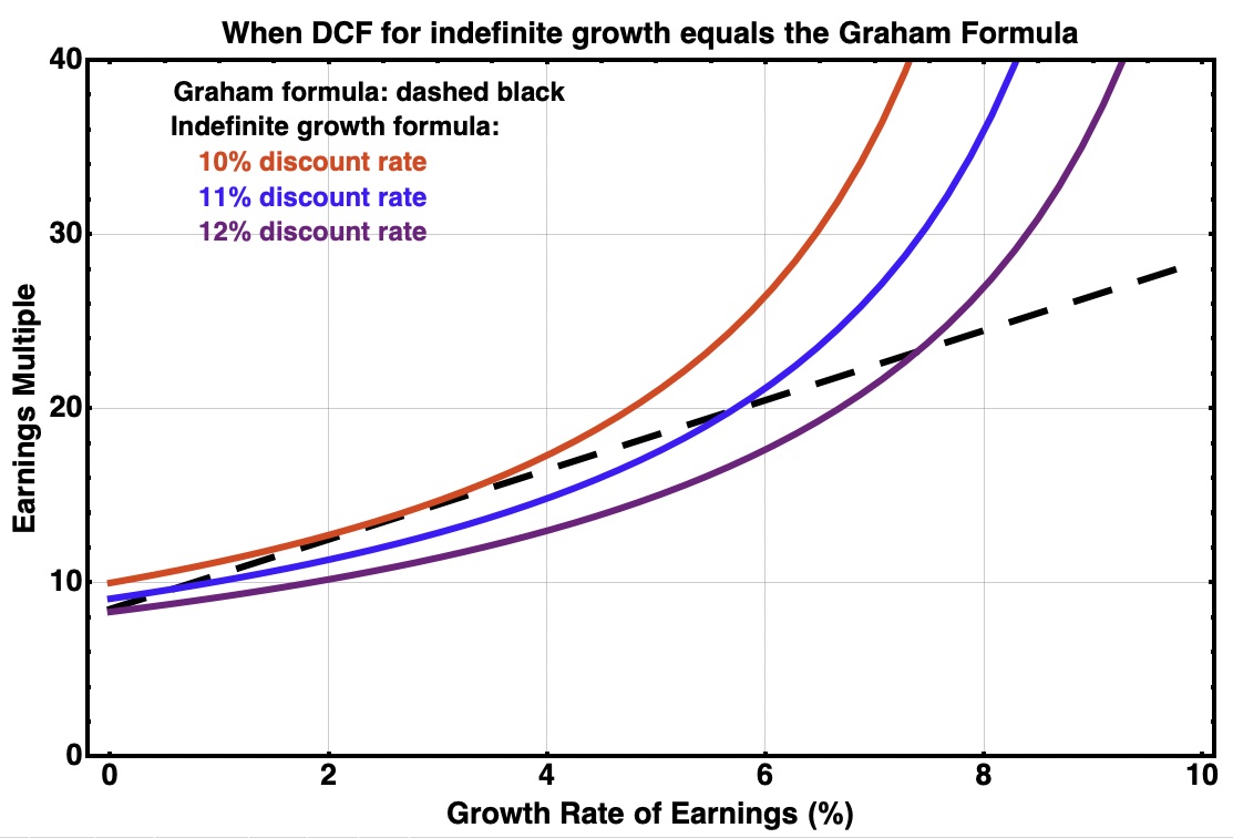
One sees that the Graham formula corresponds to a discount rate of about 10% up to a growth rate of 5%, but then the corresponding discount rate increases. It is near 12% for growth rates between 7% and 8%.

For indefinite growth, the earnings multiple diverges upward as the discount rate approaches the growth rate. One can see this by comparing the values of the colored curves above at some growth rate. For example, at a growth rate of 7%, the multiple for a discount rate of 10% is more than 50% larger than that for a discount rate of 12%.

This upward divergence in the indefinite-growth results reflects the role of very distant earnings and is not really sensible. It is worth somehow ignoring. Graham was aware that his model did this, and liked that aspect.

The implication of the Graham model is that larger growth rates deserve much larger discount rates in an indefinite-growth model. If we solve for the discount rate that gives equal earnings multiples from the two models, we see this:

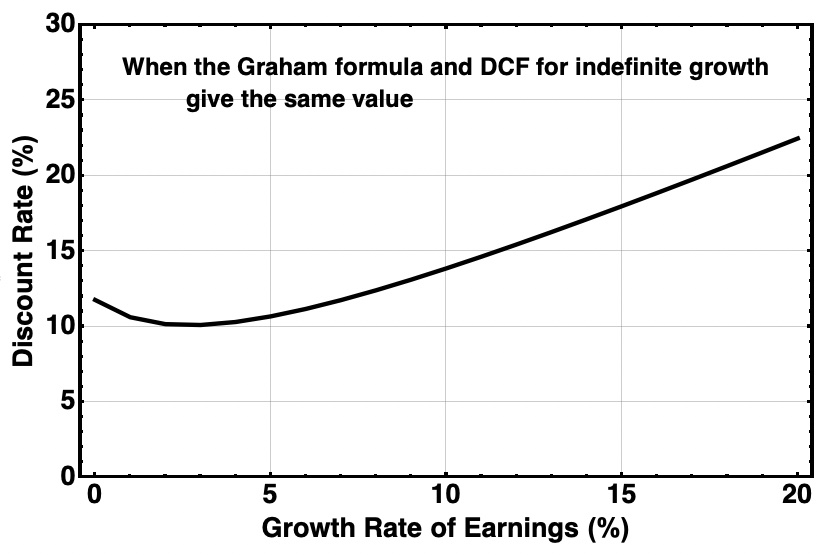
As the growth rate of earnings increases above 5%, so does the discount rate implied by the Graham model. Distant earnings are increasingly discounted. This is sensible, at least qualitatively.

Two Phase Growth Models

But still, the Graham model seems a rather crude way to deal with really large growth rates. What author Martin does has three parts and is called the Martin/Graham model below.

He first uses an explicit earnings model to find the anticipated mid-cycle earnings after 7 years. Then he applies the Graham formula with a 7% growth rate to determine the implied fair value at that time.

Martin then looks at the implied CAGR to get from the current price to that fair value after 7 years. This is the return on the investment in the absence of dividends.

To include dividends we can use the Gordon Growth Model and add the CAGR of fair value to the dividend yield. This appeals to me as an investor in REITs and MLPs, where much of the return comes in the form of dividends or distributions.

To my mind this is a better approach than just applying the Graham formula to the current growth rate. I developed a variation of this approach when considering investments in MegaCap Tech stocks last year, as discussed here.

Another thing that appeals to me about the approach of Martin is that it gives a very clear estimate of total return. The simple, indefinite-return model has the simple interpretation that the discount rate is the total return.

This works well for a fixed growth rate. But the relation of discount rate and total return becomes more fuzzy when the growth rate is adjusted over time. Besides, one cares most about the total return (based on fair value) over some period of time from the present.

The Math and Results For High Growers

We can implement this Martin/Graham model mathematically as is shown here:

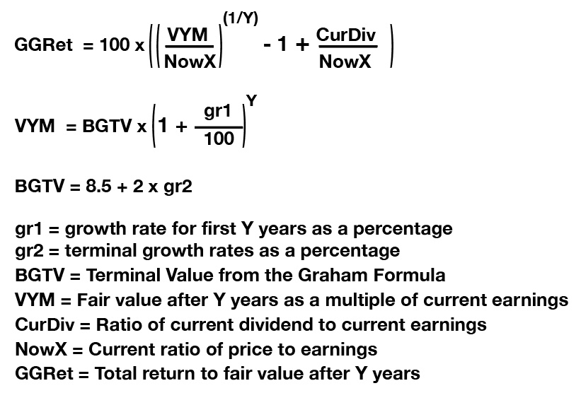
In applying this to growth stocks that pay no dividend, one would set the variable CurDiv to zero. In contrast, for stocks where the returns of interest are entirely in the form of dividends, one would set it to one.

Graham and Martin both recommend using no higher than a 20% growth rate for earnings in finding a valuation, as higher values have proven difficult to sustain. We can do this and compare cases with no dividends and where 30% of earnings is paid out as dividends, obtaining the following:

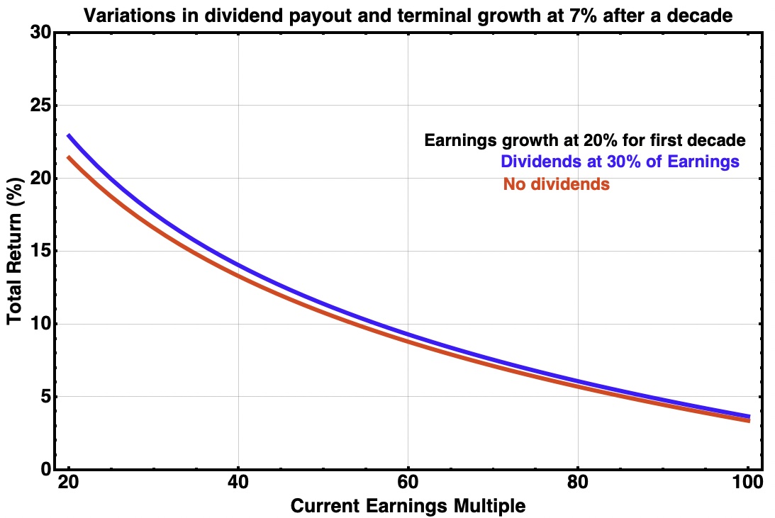
Martin’s hurdle rate is a 12% return. To meet it, one should pay no more than about 45 times (midcycle) earnings for a company whose earnings seem sure to grow for a decade at 20%.

It is notable that an investor’s total return is typically less than the initial, rapid rate of earnings growth. This reflects the current pricing of that growth by the market.

But perhaps the earnings growth will be somewhat slower. Here is a comparison of 15% vs 20% initial earnings growth, with the 12% return hurdle rate shown as a dashed line.

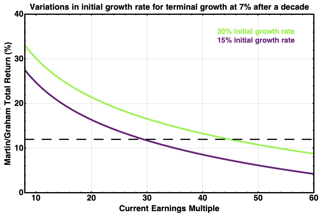
The firm that will grow earnings at 15% deserves a lot lower multiple than one which will do 20%. At Martin’s hurdle rate, the variation is from an earnings multiple of 30 to one of 45.

Results for Slower Growth

Pass-through, high-dividend entities such as REITs and MLPs pay out most of their earnings as distributions. These firms grow more slowly most of the time.

Their earnings yield is only somewhat larger than their dividend yield. For REITs the difference is typically 25% of the dividend.

We look first at the impact of the terminal growth rate, which shows the effect of distant earnings. This graphic assumes 7% growth for the first decade.

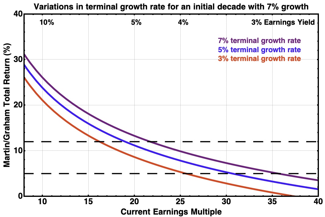
The difference between a terminal growth rate of 7% and 3% is about 5% in total return. This is not negligible.

Few REITs or MLPs are likely to grow indefinitely at 7% or more [although AvalonBay (AVB) has managed 7.7% for some decades]. But it is not hard to get to 5%, so we use that going forward.

Here we show total returns against earnings multiple for initial growth rates of 5% to 10%:

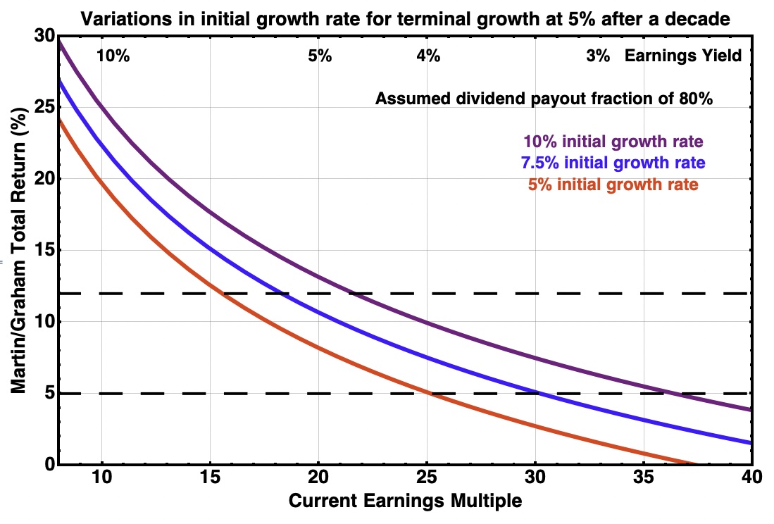
REITs have tended to produce economic total returns (the sum of earnings growth and dividend yield) in the range of 5% to 12% in normal markets. The horizontal dashed lines show these values.

Last year quite a few popular REITs were priced at earnings multiples well up into the 30s. Here we take the earnings multiple as Price/AFFO, where AFFO is Adjusted Funds From Operations, discussed here.

This reflected the extreme demand for property whose rents and value were able to keep up with inflation. Let’s consider the impact on REITs. (There are similarities for MLPs and midstream corporations.)

REITs will see an increase in nominal earnings with inflation. In some cases this will be direct and seen in revenue.

In other cases it will reflect increased property values, which can power increases in earnings growth. As an example, in a recent earnings call AvalonBay discussed adding debt to stay leverage-neutral as their earnings and property values increased.

One could incorporate some related assumptions into the earnings projection for a specific Martin/Graham model. In general, though, the impact of inflation will be to push the results upward on the graphic above.

As an example, a 7.5% grower who will also benefit from 5% inflation might hit a nominal total return a couple percent above the purple curve. From this perspective, for quality REITs priced in the mid-30s one could say that the market will accept a nominal total return in the high-single digits through a combination of real economic growth and anticipated inflation.

Some Opportunistic REITs

In the wake of this year’s bear market, there are quite a few better opportunities today. Here is a table of several REITs with high credit ratings, showing how far they have dropped in price and the ratio of price to estimated 2022 AFFO (from TIKR).

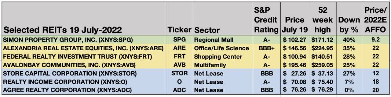
The row shaded green shows Simon Property Group (SPG), by far the best value in the market for a blue-chip REIT today, being priced at 9.2x AFFO. Simon is unlikely to grow at high rates, but is likely to do at least 5%. Their historical average has been higher than that.

SPG is priced to earn you above 20% total returns, even if the growth rate falls somewhat below 5%. The only reason not to own this stock is if you have apocalyptic visions of their future.

(Since someone will ask, Macerich (MAC) is not a blue-chip, is saddled by debt that puts them years away from significant growth, and has a history of diluting shareholders. I see SPG as a better choice.)

The rows shaded gold show three blue-chip REITs that have all dropped substantially and are now priced at about 22x AFFO. If they can grow earnings at rates about 7.5% for the next decade, and ignoring inflation, the Martin/Graham framework projects a total return above 10%.

This is an interesting result. These three REITs were priced at or above 30x last year. If you think they will go back there, the upside is around 50% and the total return getting there is likely to far exceed 10%. Whether you get 10% or a lot more will reflect the evolution in how highly the market values cash flows and how much it anticipates inflation.

The rows shaded blue compare three “Net Lease” REITs. Here we see a huge disconnect. STORE Capital (STOR) is priced at 12x AFFO and has dropped 27% in price. In contrast, Realty Income (O) and Agree Realty (ADC) are priced at or above 18x and have dropped little.

The market seems to have bought the line that STORE is vulnerable because their tenants do not carry investment-grade credit ratings. In my view, and after a lot of research, this argument holds no water. The results support that point of view.

But even if one buys the argument, does STOR deserve to be priced at a 33% discount to the other two? This is not credible.

The business model of STORE will enable earnings growth in that 7.5% ballpark (and sometimes more). The Martin/Graham model then says that STOR is priced for total returns around 18%.

Yet we see articles advocating that investors buy O and ADC today. Sorry, but that’s probably not so smart. Buy STOR. You will be glad you did.

Wrapping Up

It has been deeply interesting to learn the details about Graham’s valuation model. The way that Martin incorporated it into a valuation method seems pretty compelling to me.

It has also been interesting to work out the model presented here and to compare it with past models I’ve done. The value of stocks in firms that face a decade of very rapid growth is mainly anchored in that decade.

In contrast, the pricing of cash flows from real estate very much includes payment for cash flows in the fairly distant future. The present value is strongly affected by how one assesses that.

With my goal of achieving total returns well above 10%, this research has increased my skepticism of very high earnings multiples for REITs. My point of view at this moment is as follows: If any REIT you buy near 20x gets above 30x, it may be time to sell.