

Olivier Le Moal
Executive Summary
Firms such as Bridgewater Associates pioneered the concept of “risk parity”, allocating assets in a way that balances their risk contribution to the overall portfolio risk. Underpinning this strategy is the assumption that higher volatility in an asset should result in a lower weight, and vice versa. However, outside of equities, the relationship between volatility and return is not nearly as clear-cut. Acknowledging a variable relationship between the two for other assets has the potential not only to improve risk-adjusted returns but lead to more diversity from the herd in managing portfolio changes in the future.
For decades, the 60-40 portfolio has been the gold standard for investors. Easy to understand and rooted in basic principles of diversification, it allocates 60% to equities and 40% to bonds. However, naively allocating 60-40 does not directly consider the relationship between returns and volatility. Most investors are taught that volatility is always “bad” for your portfolio – but this may not always be the case.
Generally, investors are taught to seek the highest return per unit of risk in their portfolio, often simply measured using the Sharpe ratio. The goal is to improve the risk-return trade-off and smooth out portfolio returns over time. Instead of a static allocation like 60-40, a risk-focused approach will use asset volatilities and correlations to adjust portfolio weights. But this typically assumes a consistent (inverse) link between higher volatility and lower prices across assets, even if it considers the correlations among them in the process.
The inverse relationship between stock prices and volatility was first formally proposed by Fischer Black back in 1976.1 Black argued that negative equity returns increased the firm’s financial leverage with debt remaining fixed, leading to more uncertainty regarding its future value and a spike in volatility. Known as the “leverage effect”, the strong link between stock market sell-offs and higher volatility is now well-known and reinforced in financial media with the popularity of measures like the Cboe Volatility Index (VIX).2 But how does this relationship hold across asset classes when constructing a diversified portfolio? Does this “leverage effect” extend to other assets, or is the relationship different?
While most investors are accustomed to volatility spiking on big drops in the stock market, the relationship between volatility and return in other assets besides equities is much weaker or even inverted – h/phew volatility can be associated with higher returns. Acknowledging this potential difference can help enhance some of the traditional risk-focused approaches to asset allocation, especially when long-held assumptions start to be challenged by big current shifts in the market.
Sophisticated asset managers such as Bridgewater and AQR have championed risk-focused approaches to asset allocation for decades, often under the umbrella term of “risk parity”. While a traditional portfolio may have only 60% allocated to equities, that portion can represent about 90% of the portfolio risk.3 A risk parity approach seeks to achieve more balance by allocating according to risk, reducing weight in riskier, more volatile assets and allocating more (or leveraging) in lower-volatility assets, looking to improve risk-adjusted returns no matter what the market environment.
Risk-First Portfolio Construction
For this analysis, we simplify this style of investing into two broad strategies, Risk Parity (RP) and Equity Risk Budget (ERB), with just two asset classes, US equities and US Treasuries. We use the trailing 252-day standard deviation of returns as the prevailing short-term volatility estimate for both stocks (E) and bonds (B).4 Also for simplicity, we assume the long-term volatility of each asset class is constant at 18% for equities (E,T) and 6% for bonds (B,LT)5. These estimates provide the necessary components to calculate the equity allocation (+E) using both strategies. The remainder is allocated to bonds (+ B’ 1 – E).
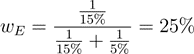
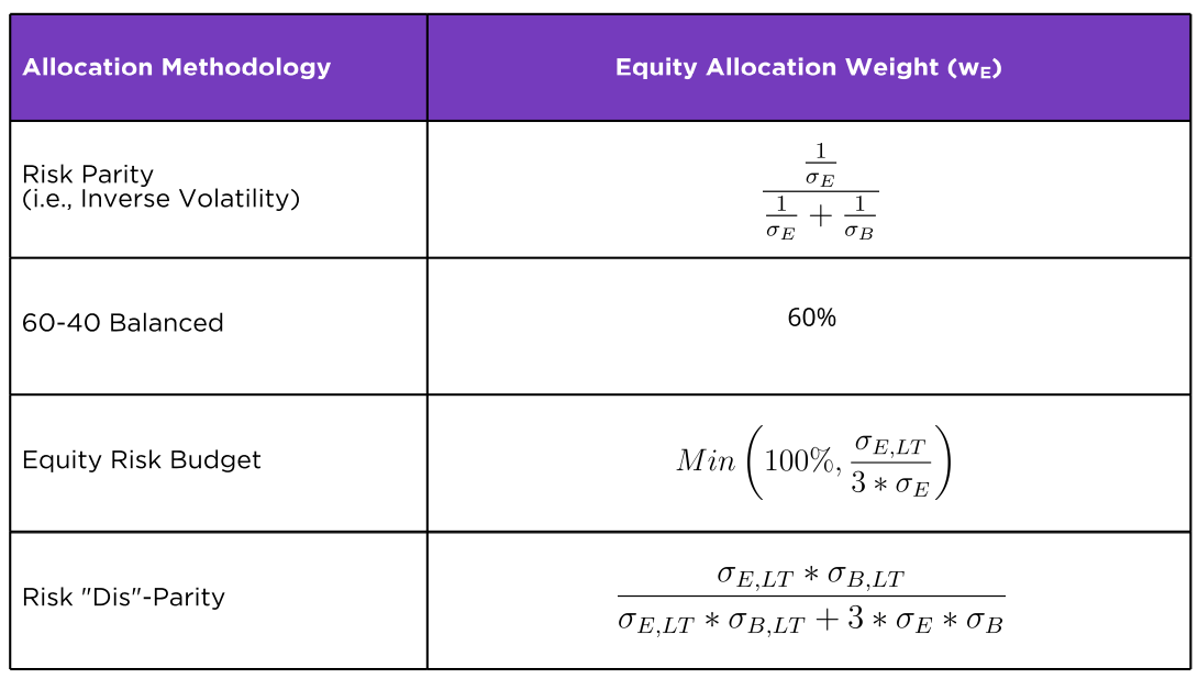
Let’s assume the prevailing short-term estimates for equity and bond volatilities are 15% and 5%, respectively. For Risk Parity, we allocate a percentage to equities that is inversely proportional to this volatility estimate as follows:
The Equity Risk Budget method uses the same short-term estimate of 15% and anchors it to the long-term estimate of 18%, allocating it as follows:
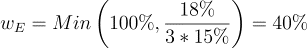
The “3” in the denominator is based on our assumption that equities are roughly three times more volatile than bonds (18%/6%) over the long term.6 The ERB method results in a more aggressive allocation to equities relative to the Risk Parity approach. And of course, the benchmark 60-40 portfolio simply allocates +E’ 60%.
These allocation strategies make certain other assumptions. Chief among them is that equities and bonds behave similarly in the presence or absence of volatility. High volatility typically begets more volatility and is seen as a precursor for lower risk-adjusted returns, prompting us to allocate less. Conversely, low volatility is seen as an advantageous time to invest, so we allocate more. Simply put, asset volatility and returns are assumed to have a negative correlation, resulting in higher weight for lower-volatility assets, and vice versa.
However, the evidence suggests this leverage effect may not exist for lower-risk assets such as US Treasuries and other government debt (as confirmed in Figure 1 below), and is weaker for other assets classes such as commodities and foreign exchange.7
Figure 1: Leverage Effect
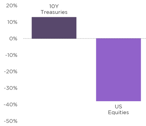
Note: This figure illustrates the leverage effect by measuring the correlation between the monthly variance and the monthly return. These are measured as the variance of the daily returns within a given month and the monthly return, respectively. See footnote 9 for more information on the underlying time series.
If higher volatility in Treasuries may, in fact, be associated with higher risk-adjusted returns for government bonds, the relative weighting between equities and bonds can be optimized to reflect this perspective.
Introducing Risk ”Dis”-Parity
To exploit the positive relationship between Treasury volatility and returns, we allocate equities inversely proportional to equity volatility and bonds proportionally to bond volatility. We call this approach Risk “Dis”-Parity (RDP), a modification of the classic Risk Parity. It still allocates based on risk rather than capital, much like Risk Parity, but in a dissimilar way that capitalizes on the empirical relationships between risk and return for these two assets rather than the theoretical justification.8
No further volatility estimations are necessary to calculate the portfolio allocation for Risk Dis-Parity. With the same assumptions, the RDP weighting would be calculated as follows:
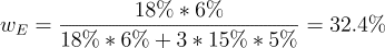
As with the ERB example above, this also assumes that equities are three times more volatile than bonds over the long term, removing the reliance on a user-specified volatility target (for the raw formulas with the notation intact, please see the Appendix).
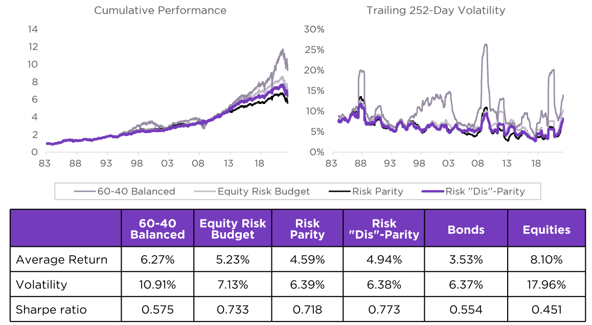
Figure 2: Strategy Performance
No single risk-focused strategy presented thus far is definitively right or wrong. It comes down to the investment objective along with the underlying assumptions regarding how asset class returns respond to volatility. If we look at the data and alter our assumptions with respect to fixed income – at least for lower-risk government bonds – we can construct risk-focused portfolios that can potentially boost risk-adjusted returns while adding benefits that go beyond the Sharpe ratio.
Performance
Even the most robust and consistent strategies will suffer bouts of underperformance and will continue to have them in the future, making it difficult to definitively evaluate the performance advantage. However, historical data is the only lens available to evaluate this (or any other) strategy. Using data from back to 1982, we test the efficacy of Risk Dis-Parity by forming portfolios on a daily basis using all four asset allocation methods.9
From Figure 2, the Sharpe ratio for the 60-40 portfolio (0.575) is marginally higher than that of Bonds (0.554) but with a much higher average return, a welcome benefit from diversification and an illustration of the efficient frontier. However, the risk-focused allocation methods are all significantly higher (by about 25%).
Risk Dis-Parity registers the highest Sharpe ratio at 0.773. In second place, despite only considering equity volatility, the Equity Risk Budget methodology records a Sharpe ratio of 0.733. Finally, Risk Parity trails slightly with a Sharpe ratio of 0.718.
The 60-40 portfolio’s performance is handicapped by not having an eye on risk. Investors are subject to wild swings which generally occur during market-wide volatility events. On the other hand, the three risk-focused strategies combat elevated market volatility by dynamically changing the portfolio allocation through a risk-focused lens. Investing 60% in equities during the Global Financial Crisis does not have the same risk profile as in 2017 when volatility was at record lows.
RDP appears to stand on its own as an attractive asset allocation strategy. But it also performs well when using a volatility targeting mechanism as an added layer of risk management. With volatility targeting, also known as risk control, volatilities and correlations are used not just for asset allocations but for dynamically adjusting the portfolio with cash or leverage to target a specified level of volatility.
Risk control is effectively doubling down on the leverage effect. For each risk-focused strategy, we assess the risk-reward trade-off at an asset class level to determine the relative weightings (i.e., +E and + BJ, as presented above. The same risk-reward trade-off is also considered at the portfolio level. Higher portfolio volatility results in lower (equity and bond) exposure, and vice versa. For Risk Dis-Parity, this counteracts the dynamic of increasing bond exposure as bond volatility rises. However, given equities contribute the majority of portfolio risk, this impact is muted in this portfolio-level leverage effect.
Turning to Figure 3, Risk Dis-Parity remains the top performer with a Sharpe ratio of 0.794, benefitting directly from the risk control overlay. Interestingly, the risk control overlay improves Risk Parity the most from the base strategy with no volatility targeting, shifting to the second spot ahead of the Equity Risk Budget methodology. The small edge in Sharpe ratio for RDP is certainly a positive, but there are also secondary benefits in using this method of risk-focused allocation versus the two alternatives.
Figure 3: Risk-Controlled Strategy Performance
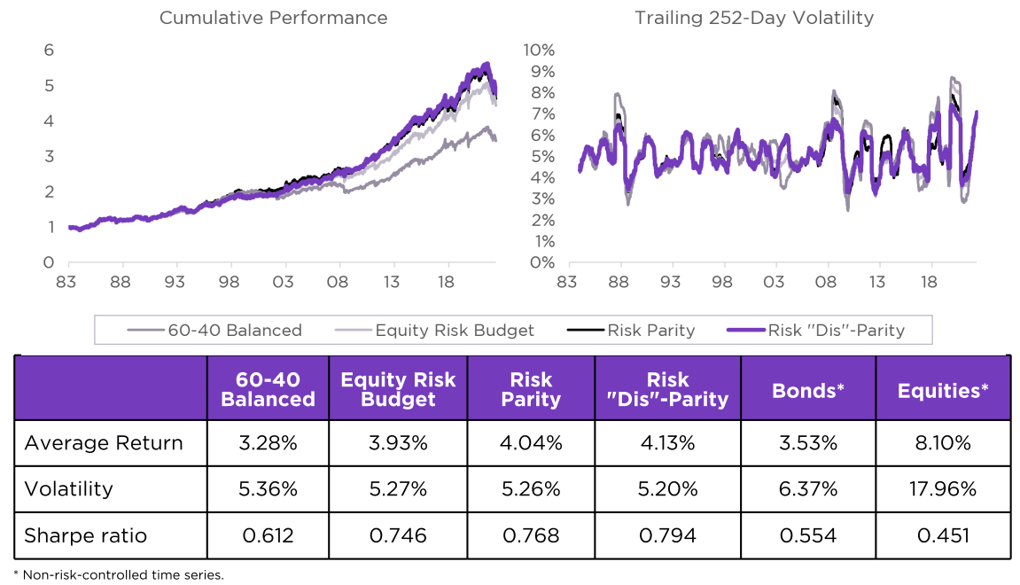
Risk Dis-Parity demonstrates lower reliance on bond returns for performance. The historical average bond weight was 67.2% for Risk Parity and only 61.5% for Risk Dis-Parity, a difference of nearly six percentage points. Even with the lower exposure to bonds over a very strong period for fixed income, Risk Dis-Parity still managed to edge out Risk Parity in performance. With the potential for interest rates to climb higher, capturing performance away from the fixed income allocation is likely a desirable trait. A lower bond allocation suggests the potential to outperform in the future if the rate environment proves to be challenging by leaning on other asset classes to contribute higher returns.
Risk Dis-Parity provides diversity for a potentially crowded strategy. Looking at the risk-controlled versions of RDP and RP, equity weight changes are 82% correlated, while the bond weight changes are only 45% correlated. If there are significant assets tied to largely similar versions of Risk Parity, they will tend to be on the same side of the trade, leading to higher transaction costs as the strategy regularly rebalances. With Risk Dis-Parity, some of the rebalancing activity may be on the other side of those trades, potentially taking advantage of more favorable prices.
Risk Dis-Parity historically delivers more stable index volatility. The volatility of volatility, or “vol-of-vol”, was the lowest among all risk-controlled versions of the strategies (0.80% for RDP versus 0.87% for RP; 0.96% for ERB; and 1.19% for the 60-40). This is attractive because it can help with pricing on derivatives linked to the index used in products such as fixed-index annuities. Lower vol-of-vol gives a dealer more confidence in the stability of the realized volatility of the index, which can lead to a lower option price, benefitting the end-investor allocated to the strategy.10
Conclusion
For decades, investors have been associating high volatility with low returns and vice versa for both equities and bonds. However, the empirical data suggests these relationships can vary by asset class. The evidence for equities appears robust – negative returns results in more firm leverage, leading to higher volatility. But this same reasoning does not necessarily apply to bonds, as some academic research clearly documents. In fact, high bond volatility, at least for Treasuries, may actually be a good thing and lead to higher risk-adjusted returns.
The simplified version of the risk-focused asset allocation strategy we call Risk “Dis”-Parity outlined above is just a starting point. Equities may have the strongest negative relationship between price and volatility and government bonds the strongest positive one, but other asset classes fall somewhere in the middle. For example, corporate credit shows the same negative correlation to volatilities as equities but is much weaker. Commodities and certain FX pairs behave similarly to government bonds, experiencing rallies while their volatilities tick higher.11
A more balanced strategy like Risk Parity can be an effective tool for investors over the long term and has attracted significant institutional assets. But some tweaking of the asset allocation using this concept of Risk Dis-Parity that acknowledges the risk/return relationship may not be uniform across assets may provide improvements and potential to outperform.
Appendix
The following table outlines the formulas for the equity allocation under each scenario.
Disclosures
Copyright 2022 Salt Financial Indices LLC.Salt Financial Indices LLC is a division of Salt Financial LLC. “Salt Financial” and “TRUVOL” are registered trademarks of Salt Financial Indices LLC.
All information provided by Salt Financial Indices is impersonal and not tailored to the needs of any person, entity or group of persons. Salt Financial Indices receives compensation in connection with licensing its content (“Data”) contributed to third parties for use in an index. Past performance of an index is not a guarantee of future results. Salt Financial Indices is not an investment advisor and makes no representation regarding the advisability of investing in any such investment fund or other investment vehicle.
These materials have been prepared solely for informational purposes based upon information generally available to the public and from sources believed to be reliable. Salt Financial Indices and its third-party data providers and licensors (collectively, the “Salt Financial Indices LLC Parties”) do not guarantee the accuracy, completeness, timeliness or availability of the Data. The Salt Financial Indices LLC Parties are not responsible for any errors or omissions, regardless of the cause, for the results obtained from the use of the Data. The Data is provided on an “as-is” basis. In no event shall the Salt Financial Indices LLC Parties be liable to any party for any direct, indirect, incidental, exemplary, compensatory, punitive, special or consequential damages, costs, expenses, legal fees, or losses (including, without limitation, lost income or lost profits and opportunity costs) in connection with any use of the Data even if advised of the possibility of such damages.
________
Footnotes:
1 Black, Fischer. “Studies of Stock Price Volatility Changes.” In. Proceedings of the /976 /’4eef/ng of the Business and Economic Stat/st/cs Sect/on, 1976, 177-81.
2 Hasanhodzic, Jasmina, and Andrew W. Lo. “On Black’s Leverage Effect in Firms with No Leverage.” 46, no. (October 3l, 2019): 106-22.
3 See “Risk Parity IS About Balance”, available here.
4 We use a historical equally-weighted standard deviation for simplicity but there are more sophisticated ways to estimate volatility, such as using an exponentially weighted moving average (EWMA) or via higher-frequency realized volatility data. See our research note “The Layman’s Guide to Volatility Forecasting” for a more detailed overview.
5 Long-term volatilities are estimated using Bloomberg data from May 1982 – September 2022. The advantage of incorporating long-term volatilities into these calculations eliminates the need to arbitrarily select a “volatility target”. These long-term volatilities are only relevant for Equity Risk Budgeting and Risk “Dis”-Parity. The 60-40 and Risk Parity portfolios do not rely on a volatility target.
6 The long-term ratio of equity to bond volatility is relatively consistent at 3:1 but linking it to a more dynamic long-term trailing ratio of stock to bond volatility can be easily substituted to account for any future changes in that relationship.
7 Harvey, Campbell R., Edward Hoyle, Russell Korgaonkar, Sandy Rattray, Matthew Sargaison, and Otto Van Hemert. “The Impact of Volatility Targeting.”The Journal of Portfolio Management 45, no. I (2018): 14-33.
8 Asness, Clifford S., Andrea Frazzini, and Lasse H. Pedersen. “Leverage Aversion and Risk Parity.”6/nanc/a/ Analysis Journal 68, no. (2012): 47-59.
9 We source long-dated indices from Bloomberg to represent equities and bonds. The equity component is represented by the Russell 1000 Total Return Index (ticker: RU10INTR Index), and the bond component is tracked by the Merrill Lynch 10Y US Treasury Tracker Total Return Index (ticker: MLT1US10 Index}. Data is from May 1982 through September 2022.
10 In the case of fixed-indexed annuities, the investor is generally a retiree. They are investing in the annuity for the principal protection and index-linked upside. A cheaper option price provides them more upside, ultimately resulting in higher annual index-linked credits for their account.
11 Harvey, Campbell R., Edward Hoyle, Russell Korgaonkar, Sandy Rattray, Matthew Sargaison, and Otto Van Hemert. “The Impact of Volatility Targeting.” The Journal of Portfolio Management 45, no. 1 (2018}: 14-33.
Editor’s Note: The summary bullets for this article were chosen by Seeking Alpha editors.
Be the first to comment